Continuous Random Variables Are Obtained From Data That Can Be Measured Rather Than Counted

Two Types of Random Variables

A random variable

$\text{x}$

, and its distribution, can be discrete or continuous.

Learning Objectives

Contrast discrete and continuous variables

Key Takeaways

Key Points

• A random variable is a variable taking on numerical values determined by the outcome of a random phenomenon.
• The probability distribution of a random variable

  $\text{x}$

  tells us what the possible values of

  $\text{x}$

  are and what probabilities are assigned to those values.
• A discrete random variable has a countable number of possible values.
• The probability of each value of a discrete random variable is between 0 and 1, and the sum of all the probabilities is equal to 1.
• A continuous random variable takes on all the values in some interval of numbers.
• A density curve describes the probability distribution of a continuous random variable, and the probability of a range of events is found by taking the area under the curve.

Key Terms

• random variable: a quantity whose value is random and to which a probability distribution is assigned, such as the possible outcome of a roll of a die
• discrete random variable: obtained by counting values for which there are no in-between values, such as the integers 0, 1, 2, ….
• continuous random variable: obtained from data that can take infinitely many values

Random Variables

In probability and statistics, a randomvariable is a variable whose value is subject to variations due to chance (i.e. randomness, in a mathematical sense). As opposed to other mathematical variables, a random variable conceptually does not have a single, fixed value (even if unknown); rather, it can take on a set of possible different values, each with an associated probability.

A random variable's possible values might represent the possible outcomes of a yet-to-be-performed experiment, or the possible outcomes of a past experiment whose already-existing value is uncertain (for example, as a result of incomplete information or imprecise measurements). They may also conceptually represent either the results of an "objectively" random process (such as rolling a die), or the "subjective" randomness that results from incomplete knowledge of a quantity.

Random variables can be classified as either discrete (that is, taking any of a specified list of exact values) or as continuous (taking any numerical value in an interval or collection of intervals). The mathematical function describing the possible values of a random variable and their associated probabilities is known as a probability distribution.

Discrete Random Variables

Discrete random variables can take on either a finite or at most a countably infinite set of discrete values (for example, the integers). Their probability distribution is given by a probability mass function which directly maps each value of the random variable to a probability. For example, the value of

$\text{x}_1$

takes on the probability

$\text{p}_1$

, the value of

$\text{x}_2$

takes on the probability

$\text{p}_2$

, and so on. The probabilities

$\text{p}_\text{i}$

must satisfy two requirements: every probability

$\text{p}_\text{i}$

is a number between 0 and 1, and the sum of all the probabilities is 1. (

$\text{p}_1+\text{p}_2+\dots + \text{p}_\text{k} = 1$

)

Discrete Probability Disrtibution: This shows the probability mass function of a discrete probability distribution. The probabilities of the singletons {1}, {3}, and {7} are respectively 0.2, 0.5, 0.3. A set not containing any of these points has probability zero.

Examples of discrete random variables include the values obtained from rolling a die and the grades received on a test out of 100.

Continuous Random Variables

Continuous random variables, on the other hand, take on values that vary continuously within one or more real intervals, and have a cumulative distribution function (CDF) that is absolutely continuous. As a result, the random variable has an uncountable infinite number of possible values, all of which have probability 0, though ranges of such values can have nonzero probability. The resulting probability distribution of the random variable can be described by a probability density, where the probability is found by taking the area under the curve.

Probability Density Function: The image shows the probability density function (pdf) of the normal distribution, also called Gaussian or "bell curve", the most important continuous random distribution. As notated on the figure, the probabilities of intervals of values corresponds to the area under the curve.

Selecting random numbers between 0 and 1 are examples of continuous random variables because there are an infinite number of possibilities.

Probability Distributions for Discrete Random Variables

Probability distributions for discrete random variables can be displayed as a formula, in a table, or in a graph.

Learning Objectives

Give examples of discrete random variables

Key Takeaways

Key Points

• A discrete probability function must satisfy the following:

  $0 \leq \text{f}(\text{x}) \leq 1$

  , i.e., the values of

  $\text{f}(\text{x})$

  are probabilities, hence between 0 and 1.
• A discrete probability function must also satisfy the following:

  $\sum \text{f}(\text{x}) = 1$

  , i.e., adding the probabilities of all disjoint cases, we obtain the probability of the sample space, 1.
• The probability mass function has the same purpose as the probability histogram, and displays specific probabilities for each discrete random variable. The only difference is how it looks graphically.

Key Terms

• discrete random variable: obtained by counting values for which there are no in-between values, such as the integers 0, 1, 2, ….
• probability distribution: A function of a discrete random variable yielding the probability that the variable will have a given value.
• probability mass function: a function that gives the relative probability that a discrete random variable is exactly equal to some value

A discrete random variable

$\text{x}$

has a countable number of possible values. The probability distribution of a discrete random variable

$\text{x}$

lists the values and their probabilities, where value

$\text{x}_1$

has probability

$\text{p}_1$

, value

$\text{x}_2$

has probability

$\text{x}_2$

, and so on. Every probability

$\text{p}_\text{i}$

 is a number between 0 and 1, and the sum of all the probabilities is equal to 1.

Examples of discrete random variables include:

• The number of eggs that a hen lays in a given day (it can't be 2.3)
• The number of people going to a given soccer match
• The number of students that come to class on a given day
• The number of people in line at McDonald's on a given day and time

A discrete probability distribution can be described by a table, by a formula, or by a graph. For example, suppose that

$\text{x}$

is a random variable that represents the number of people waiting at the line at a fast-food restaurant and it happens to only take the values 2, 3, or 5 with probabilities

$\frac{2}{10}$

,

$\frac{3}{10}$

, and

$\frac{5}{10}$

respectively. This can be expressed through the function

$\text{f}(\text{x})= \frac{\text{x}}{10}$

,

$\text{x}=2, 3, 5$

or through the table below. Of the conditional probabilities of the event

$\text{B}$

given that

$\text{A}_1$

is the case or that

$\text{A}_2$

is the case, respectively. Notice that these two representations are equivalent, and that this can be represented graphically as in the probability histogram below.

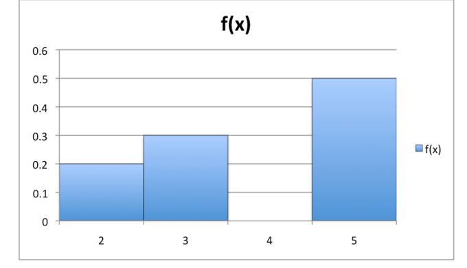
Probability Histogram: This histogram displays the probabilities of each of the three discrete random variables.

The formula, table, and probability histogram satisfy the following necessary conditions of discrete probability distributions:

1. $0 \leq \text{f}(\text{x}) \leq 1$

   , i.e., the values of

   $\text{f}(\text{x})$

   are probabilities, hence between 0 and 1.

2. $\sum \text{f}(\text{x}) = 1$

   , i.e., adding the probabilities of all disjoint cases, we obtain the probability of the sample space, 1.

Sometimes, the discrete probability distribution is referred to as the probability mass function (pmf). The probability mass function has the same purpose as the probability histogram, and displays specific probabilities for each discrete random variable. The only difference is how it looks graphically.

Probability Mass Function: This shows the graph of a probability mass function. All the values of this function must be non-negative and sum up to 1.

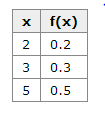
Discrete Probability Distribution: This table shows the values of the discrete random variable can take on and their corresponding probabilities.

Expected Values of Discrete Random Variables

The expected value of a random variable is the weighted average of all possible values that this random variable can take on.

Learning Objectives

Calculate the expected value of a discrete random variable

Key Takeaways

Key Points

• The expected value of a random variable

  $\text{X}$

  is defined as:

  $\text{E}[\text{X}] = \text{x}_1\text{p}_1 + \text{x}_2\text{p}_2 + \dots + \text{x}_\text{i}\text{p}_\text{i}$

  , which can also be written as:

  $\text{E}[\text{X}] = \sum \text{x}_\text{i}\text{p}_\text{i}$

  .
• If all outcomes

  $\text{x}_\text{i}$

  are equally likely (that is,

  $\text{p}_1=\text{p}_2=\dots = \text{p}_\text{i}$

  ), then the weighted average turns into the simple average.
• The expected value of

  $\text{X}$

  is what one expects to happen on average, even though sometimes it results in a number that is impossible (such as 2.5 children).

Key Terms

• discrete random variable: obtained by counting values for which there are no in-between values, such as the integers 0, 1, 2, ….
• expected value: of a discrete random variable, the sum of the probability of each possible outcome of the experiment multiplied by the value itself

Discrete Random Variable

A discrete random variable

$\text{X}$

has a countable number of possible values. The probability distribution of a discrete random variable

$\text{X}$

lists the values and their probabilities, such that

$\text{x}_\text{i}$

has a probability of

$\text{p}_\text{i}$

. The probabilities

$\text{p}_\text{i}$

must satisfy two requirements:

1. Every probability

   $\text{p}_\text{i}$

   is a number between 0 and 1.
2. The sum of the probabilities is 1:

   $\text{p}_1+\text{p}_2+\dots + \text{p}_\text{i} = 1$

   .

Expected Value Definition

In probability theory, the expected value (or expectation, mathematical expectation, EV, mean, or first moment) of a random variable is the weighted average of all possible values that this random variable can take on. The weights used in computing this average are probabilities in the case of a discrete random variable.

The expected value may be intuitively understood by the law of large numbers: the expected value, when it exists, is almost surely the limit of the sample mean as sample size grows to infinity. More informally, it can be interpreted as the long-run average of the results of many independent repetitions of an experiment (e.g. a dice roll). The value may not be expected in the ordinary sense—the "expected value" itself may be unlikely or even impossible (such as having 2.5 children), as is also the case with the sample mean.

How To Calculate Expected Value

Suppose random variable

$\text{X}$

can take value

$\text{x}_1$

with probability

$\text{p}_1$

, value

$\text{x}_2$

with probability

$\text{p}_2$

, and so on, up to value

$\text{x}_i$

with probability

$\text{p}_i$

. Then the expectation value of a random variable

$\text{X}$

 is defined as:

$\text{E}[\text{X}] = \text{x}_1\text{p}_1 + \text{x}_2\text{p}_2 + \dots + \text{x}_\text{i}\text{p}_\text{i}$

, which can also be written as:

$\text{E}[\text{X}] = \sum \text{x}_\text{i}\text{p}_\text{i}$

.

If all outcomes

$\text{x}_\text{i}$

are equally likely (that is,

$\text{p}_1 = \text{p}_2 = \dots = \text{p}_\text{i}$

), then the weighted average turns into the simple average. This is intuitive: the expected value of a random variable is the average of all values it can take; thus the expected value is what one expects to happen on average. If the outcomes

$\text{x}_\text{i}$

are not equally probable, then the simple average must be replaced with the weighted average, which takes into account the fact that some outcomes are more likely than the others. The intuition, however, remains the same: the expected value of

$\text{X}$

is what one expects to happen on average.

For example, let

$\text{X}$

represent the outcome of a roll of a six-sided die. The possible values for

$\text{X}$

are 1, 2, 3, 4, 5, and 6, all equally likely (each having the probability of

$\frac{1}{6}$

). The expectation of

$\text{X}$

is:

$\text{E}[\text{X}] = \frac{1\text{x}_1}{6} + \frac{2\text{x}_2}{6} + \frac{3\text{x}_3}{6} + \frac{4\text{x}_4}{6} + \frac{5\text{x}_5}{6} + \frac{6\text{x}_6}{6} = 3.5$

. In this case, since all outcomes are equally likely, we could have simply averaged the numbers together:

$\frac{1+2+3+4+5+6}{6} = 3.5$

.

Average Dice Value Against Number of Rolls: An illustration of the convergence of sequence averages of rolls of a die to the expected value of 3.5 as the number of rolls (trials) grows.

Licenses and Attributions

mcdonaldhicaltisee.blogspot.com

Source: https://www.coursehero.com/study-guides/boundless-statistics/discrete-random-variables/

Share this post